SELF |
New Year question from Leo |
S.B. Karavashkin |
|
|
|
SELF |
New Year question from Leo |
S.B. Karavashkin |
|
|
|
The letter from Leo to me From: xu xu xuszxu@yahoo.comTo: Sergey Karavashkin selflab@go.com, selflab@mail.ru Date: Thu, 18 Dec 2003 09:56:31 -0800 (PST) Subject: problem on divergence formula
Dear Sergey: I have a question on your divergence formula. Please see the attached file. Merry Christmas! Leo Attachment: problem.pdf
|
|
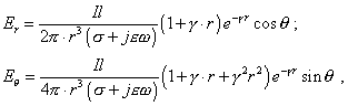
| In spherical coordinate, the electric field at point P created by a dipole Il is [1]: |
|
 |
|
| where |
|
| Obviously, the propagation direction of electric field is |
|
| (1) | |
| we have | |
| However, it can be easily verifies that | |
| I think the problem is that (1) is wrong. Reference [2]
did not consider the contribution of side-surface to the divergence of a vector when
deriving (1).
Reference [1] James R. Wait, "Introduction to antennas & propagation", Peter Peregrious Ltd, London, United Kingdom, 1986, pp 89, equation (5.30)- (5.31) [2] S.B. Karavashkin. "TRANSFORMATION OF DIVERGENCE THEOREM IN DYNAMICAL FIELDS". |
|
My respond to Leo Date: 03-12-22 Dear Leo, I think very laudable of your conception of spherical
dipole that you took from James Wait's book. However I would be much more grateful if you
analyse the derivation of the very equations by James Wait, before you compare the
expressions for divergence of flux from a spherical dipole that you give in your message
with the expression for divergence of vector in dynamic fields taken from my paper. Then
you would find interesting things that are not seen from the final formulas. Please check
attentively, and not mechanically but phenomenologically - analyse, what comes from where
and why. Then you will understand the cause. Unfortunately, I have not the book by J.
Wait, but I can help you with this analysis, basing on similar problem considered by A.M.
Kugushev [1]. In his book he also studies the electric and magnetic field of a wire with
the flowing current, whose length l << |
|
|
(1) |
where To understand the cause, let us first pay our attention
that the solution (1), just as your solutions, has been yielded by substitution of the
value of vector potential |
|
|
(2) |
i.e., in a roundabout way. First we find |
|
|
(3) |
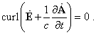
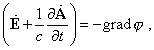
So we twice pass (1) through the filter cutting off the longitudinal component. The cause of fact that in the resulting expression this component remains is that, additionally to this all, we lose a very important summand in the expression for electric field. Actually, if in accordance with [2, p. 41] before calculating the model we substitute the first expression from (2) to the Faraday law, we will yield |
|
|
(4) |
| or | |
|
(5) |
"This last equation shows that vector |
|
 |
|
remains the potential vector. This means, we can present it as |
|
|
(6) |
| where Let us return to (6) and finish the derivation of this expression. "In distinct from the case of electrostatics, the vector of electric field having the vortex pattern already cannot be represented as the gradient of any potential. It is expressed through the assemblage of scalar and vector potentials as follows: |
|
|
(7) |
| With it the second summand that connects
the electric field with that magnetic expresses the Faraday law of electromagnetic
induction" [2, p. 42].
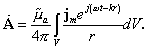
So we came to the known expression which connects scalar and vector potentials with electric field in space, and surely, no component of the field was omitted. To determine on this basis the correct relationship of electric field with respect of time and co-ordinates, we have to deviate again from our course and to pay attention to the record of vector potential. According to Kugushev, the expression for vector potential on whose basis he yielded (1) for the strength of electric field is the following [1, p. 98]: |
|
|
(8) |
We should mark, this expression is not an exact solution of the wave equation for vector potential. This will be very important for the below consideration. Really, as we know, the expression for vector potential is found on the basis of wave equation like [1, p.88] |
|
|
(9) |
where |
|
But the solution of this equation is not the function (8) which we consider but the integral function like [1, p. 89] or [3, p. 95]: |
|
|
(10) |
However, "for the region r >> l we can think all points of dipole equally distanced from the studied point of field, due to which we can re-record (10) as |
|
|
(11) |
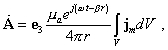
where e3 is the unit vector in direction with the current. As j m= I m /S , Sl = V and S is the cross-section of wire, we yield |
|
|
(12) |
Passing to the spherical co-ordinate system in which |
|
|
(13) |
we yield (8) which determines the vector potential at the distance r >> l " [1, p. 97]. |
|
Thus, (8) determines the vector potential only for far field, when according to [5], all parameters of the wave process have stabilised. So, when the researchers (Kugushev in that number) apply to near field the results obtained on the basis of this vector potential, this is illegal, as they violate the statement of problem. Therefrom we have to doubt (1). If (1) described the process in far field, there has to be no superposition of the field strengths with different attenuation characteristics and different phase shifts in this expression. This additionally corroborates the above statement that (1) has been derived incorrectly. To obtain the correct expression for the electric field
strength on the basis of (7), we have to determine the scalar potential |
|
|
(14) |
Taking into account that in our problem |
|
|
(15) |
| we can record | |
|
(16) |
| or, regarding (8), | |
|
(17) |
With it we can write down the summands in the right-hand part of (7) for the electric field strength in the following shape: |
|
|
(18) |
|
(19) |
Thus, |
|
|
(20) |
As we can see from this expression, the longitudinal and transverse components of the field have quite stabilised space attenuation with the rate of attenuation corresponding to the considered model. With it, the phase of the transverse component is shifted by 90o as to that longitudinal. This corroborates again that we correctly stated the calibration of electric field strength to be wrong, as the potential component of the field has its own characteristics of process of space propagation different from the transverse component. Now on the basis of corrected and, the main, complete expression for the electric field strength, let us compare the divergence of strength of this field with the results of my theorem of divergence of vector in dynamic fields [6]. (It is only some strange that, having well designed your notice, you didn't mention, this paper has been published in the international journal Archivum mathematicum, 37 (2001), 3, p. 233-243. Was it correct to refer to a paper, disregarding the publication? How do you think? ;-) ) To check, let us use the standard formula from your notice: |
|
|
(21) |
Given (20), the first term of the right-hand part will be |
|
|
(22) |
Accordingly, the second term will be |
|
|
(23) |
Whereupon |
|
|
(24) |
As we can see from (24), the divergence of electric field is not zero and the phase of its time variation is shifted by 90o as to the phase of longitudinal component. This fully corresponds to the phenomenology of process of wave propagation in space. We can easily check that the magnitude of divergence of the electric field strength vector in your problem also is in agreement with my theorem of divergence in dynamic fields. For it, let us take your (1) which you are interpreting quite right, and continue it up to the result: |
|
|
(25) |
So please enjoy comparing (24) with (25). As you see, there are no real difficulties with my theorem. Only the difficulties with the existing solutions for specific models take place. ;-) Surely, if you check so the derivation of Wait's expressions, you will yield similar result satisfying my theorem. True, additionally to this derivation, you should attentively analyse the additions introduced to the expression for vector potential because of finite conductivity of medium. If you question my theorem anyway, one can disprove it only having found the error in my proof, since theorem is primary as to all solutions of modelling equations. And this is not my wish. This is the objective principle to build any theory. First basic theorems are formed (in this case they are the conservation theorems for dynamic fields), then the mathematical technique is built, then the problems modelling specific processes are solved. Maxwell had built his system so, and we have to develop the EM theory so. I would like to mark especially, realising it or not, you raised a very important and interesting question which needs to be pondered and solved. If you have a wish to dive deeper into this subject, I would be pleased to help you. Happy New year with new knowledge, Sergey Reference:1. Kugushev, A.M. and Golubeva, N.S. The foundations of radioelectronics. The linear electromagnetic processes. Energia, Moscow, 1969, 880 pp. (Russian). 2. Levitch, V.G. The course of theoretical physics, vol.1. The State publishing of physical and mathematical literature, Moscow, 1962, 695 pp. 3. Landau, L.D. and Lifshiz, E.M. The field theory. In: Theoretical physics, vol. II. Nauka, Moscow, 1973, 504 pp. (Russian). 4. Karavashkin, S.B. On longitudinal EM waves. Chapter 1. Lifting the bans. SELF Transactions, 1 (1994), Eney Ltd., Ukraine, 118 pp. (English). http://angelfire.lycos.com/la3/selftrans/archive/archive.html#long 5. Karavashkin, S. B. and Karavashkina, O.N.Comparison of characteristics of propagation velocities of transversal acoustic waves and transversal EM waves in the near field. SELF Transactions, 3 (2003), 1, 9-17, http://angelfire.lycos.com/la3/selftrans/v3_1/contents3.html#taew 6. S. B. Karavashkin. Transformation of divergence theorem in dynamical fields. Archivum mathematicum, 37 (2001), 3, 233-243. http://angelfire.lycos.com/la3/selftrans/archive/archive.html#div |
|
 .
.