92

S.B. Karavashkin, O.N. Karavashkina

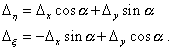
These transformations of the vibration pattern can be simply explained by the regularities of transformation from the (x, y) reference system to that (, ).

On the basis of Fig. 1 construction, the transfer conditions between the reference systems take the form

Substituting, for example, (10) and (11) into (16), we yield:

for the -component

and for the -component

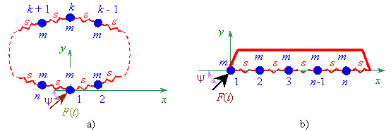
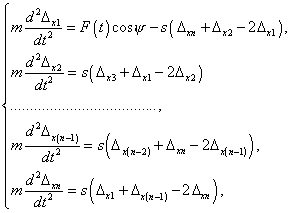
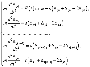
We can see from (17) and (18) that with the positive comparable with , the longitudinal -component predominates, and with the negative the transverse -component predominates. The value of longitudinal component   determines the front slop. Just due to it with the positive the front slop increases, and with that negative it diminishes.

The considered example shows that despite the bend angle does not effect on the solutions, in the specific elastic line models their own distinctions arise that are caused by the regularities of coordinate systems transformation before and after the bend point.

4. Closed-loop homogeneous elastic lumped system

Consider a closed-loop homogeneous line consisting of  n elements connected by means of elastic linear constraints having equal transverse and longitudinal stiffnesses; its general form is presented in Fig. 6a. According to the proven theorem, this line can be presented as a linear chain whose first mass is rigidly connected with the nth elastic constraint, just as it is shown in Fig. 6b. The modelling system of differential equations for this line is following:

Fig. 6. The calculation scheme of a homogeneous closed-loop elastic line consisting of n elements under the harmonic force F (t) acting with the angle to the axis x

and for the y-component

As opposite to (8)-(9), the systems of modelling equations (19)-(20) are finite, and the first and last equations of the systems (19)-(20) are connected by the cross relation through the parameters _x1, _y1 and _xn, _yn relatively. It certainly reflects on the solutions.