Acoustic field of single pulsing sphere13

V.2 No 2	13
Acoustic field of single pulsing sphere

As the second map, consider the function of the kind [8, p.150]
	(17)
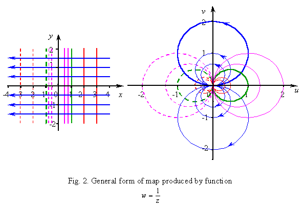
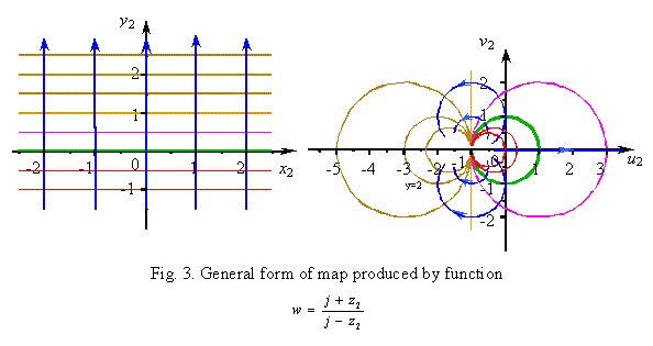
According to [8], both functions map the semi-plane inside the circumference. But we see from Fig. 2 and Fig. 3 that both functions map the entire plane z into the entire plane w . And in both cases the potential and force lines in w are the circumferences having the common point w = 0 in the first case and w = - 1 in the second. We see that these maps also do not correspond the potential field of the pulsing sphere, so we cannot use them both.


Thus the main scope of known maps is over. Let us try to model our field on the basis of non-conformal mapping. Determine the conditions which this map must satisfy. We know that the potential field surrounding the pulsing sphere is strongly radial and uniformly distributed over the angle of radiation. Furthermore, we know that in absence of pulsation the acoustic field around the sphere is absent (in distinct from EM field). As follows from this, we have to take as the prototype of model of dynamical field the metric with the uniformly distributed radial grid whose longitudinal transformation will characterise the acoustic field in space. With it the equipotential lines of non-disturbed metric must be equidistant too. The function
	(18)
satisfies these requirements. It maps non-conformally a horizontal semi-finite belt 0 y (2/b), x 0 in the plane z into the uniform radial grid in the plane w . This map is one-valued in the domain of function and multi-sheet in transition of y to the neighbouring belts y (2/b), x 0 and y (2/b), x 0 . The analytical continuation of this function is continuous. The equipotential lines in the plane z
	(19)
map within the circumference with the radius C₁x in the plane ₁. In their turn, the force lines
	(20)
map into the radial lines of plane ₁ originating from the point ₁ = ₁ = 0. The function (18) has one more peculiarity. If we change it a little and write as
	(21)
then (21) will map the above belt 0 y (2/b), x 0 into the uniform radial grid out of the circumference having radius a. So this function fully satisfies the model of stationary metric of radial field needed to construct the dynamical model.