V.2 No 2

3

Theorem of curl of a potential vector

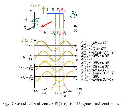
2. Preliminary analysis

As a preliminary analysis, consider a simplified model of 1D potential flux of vector vectorF.gif (853 bytes)(vectorr.gif (839 bytes), t)  whose general form is shown at the top of Fig. 2.

fig2.gif (9125 bytes)

Let in some one-connective domain omegabigcut.gif (848 bytes), free of vortexes and currents, in direction of the axis x propagate 1D homogeneous flux, whose vector vectorF.gif (853 bytes)(vectorr.gif (839 bytes), t) is normal to the direction of flux vectorn.gif (845 bytes) and the axis z. In the meanwhile we will not determine the flux as potential or vortex. For the present it will be important only that the force vector of flux is normal to the propagation direction. The item of vector solenoidality we will consider after having worked out the necessary basis.

We will suppose also that the disturbance propagation velocity is finite, and the function F(x, t) has a form

(8)

We will use again the technique used in [10] to study the divergence of vector in dynamical fields. Pick out of the studied region omegabigcut.gif (848 bytes)   three paths  ABD1E1 , ABD2E2 , ABD3E3  having the common side AB, as this is shown in Fig. 2. To visualise, choose the distance between the sides  D1E1 , D2E2 , D3E3   and the side AB equal to  2picut.gif (836 bytes)/3k ; picut.gif (836 bytes)/k ;  4picut.gif (836 bytes)/3k  relatively.

At these conditions, take the standard definition of curl of vector which, being general, must be true both for stationary and dynamical fields. This definition is the following (see, e.g., [1, p.83], [11, p.116]):
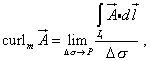
(9)

where vectorA.gif (856 bytes)  is the flux vector; P   is some point of the surface deltabig.gif (843 bytes)sigmacut.gif (843 bytes); vectorm.gif (864 bytes)  is the perpendicular to the surface deltabig.gif (843 bytes)sigmacut.gif (843 bytes); L   is the closed path bounding the surface deltabig.gif (843 bytes)sigmacut.gif (843 bytes); dvectorl.gif (848 bytes) is some infinitesimal vector element of the length of path L.

For the considered problem, (9) can be written as
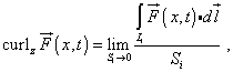
(10)

where  Si   is the cross sectional area of the ith path picked out;  i = 1, 2, 3  for ABD1E1 , ABD2E2 , ABD3E3   relatively.

As the paths picked out are finite, we first will consider the reduced circulation Ri :
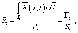
(11)
where

is the circulation of vector vectorF.gif (853 bytes)(vectorr.gif (839 bytes), t)  about the path Li .

Contents: / 1 / 2 / 3 / 4 / 5 / 6 / 7 / 8 / 9 /

Hosted by uCoz