V.2 No 1 |
77 |
| Some features of the forced vibrations modelling | |
|
|
The
considered matrix method has all above disadvantages, as it works only at the known values
|
|
|
(35) |
where a is some constant” [7, p. 296]. On the other hand, the introduction of the
main coordinates is tantamount to the simultaneous reduction of two quadratic forms T
and U to the canonical form [7, p. 266]. We can conclude from it that both matrix
methods can predict in analytical form only the fact that “if the attenuation was small, each amplitude |
|
 |
(36) |
[7, p.297]. The techniques using the Voronoy, Toeplitz and other
matrixes also have the essential drawbacks. Despite all attempts to put these matrixes in
order and to reduce them to the diagonal form, these techniques work well only if the
succession of numbers p0 > 0, p1 As a counterpoise to this, the exact analytical solutions
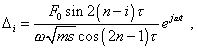
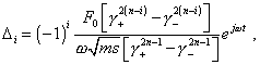
yielded by the original non-matrix method in [1] show not one but three vibration regimes:
periodical ( at |
|
|
(37) |
| at |
|
|
(38) |
| and at |
|
|
(39) |
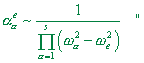
| where |
|
Comparing (37)- (39) with (36), we see them clearly determined in relation to the external force parameters, to the elastic line parameters and to the resonance frequencies. With it, when n growing, the complicacy of analysis does not increase. These solutions can be easy extended to a distributed line, which is unrealisable analytically by the matrix methods. Outwardly one can even doubt, whether (37)- (39) are reliable? As [1] shows, (37)- (39) completely satisfy the conventional modelling system of differential equations. And the aperiodical regime is not so much unexpected. The indirect methods, though they give the applicability limitation and incomplete results, in particular cases also corroborate the physical reality of this vibration regime. As an example, consider the original indirect method described by Magnus [4, pp. 282- 285]. It will be the more interesting for us that when presenting his method, Magnus studied a finite line with the fixed right end too, so we can compare the results. Magnus has drawn his attention to the relation between |
|
|
(40) |
In doing so, he naturally violated one of the boundary conditions that had to cause him the difficulties. Getting them round, he supposed that “with it in the motion equations (8) nothing will change for the individual masses, so we can seek the periodical solution having the same frequency as the excitation, and coming either in phase or in anti-phase with the excitation, supposing |
|
|
(41) |