SELF

82

S.B. Karavashkin, O.N. Karavashkina

The same as in previous example, the force affecting the interior element of line has bifurcated the solution into two intervals. In the interval  1 i k , in the periodical regime, there has arisen a standing wave having some phase delay (2k - 1)  that depends on the number of selected element k. In the interval k i the progressive wave has remained and its amplitude at the specified line parameters also depends on the number k. Hence, at

the progressive wave amplitude vanishes, and the vibrations are located in a quasi-finite section of line bounded by the line end and the external force application point. At the same time, unlike the finite line, vibrations in the quasi-finite section are non-suppressible.

These distinctions are reflected in the diagrams of Fig. 4.

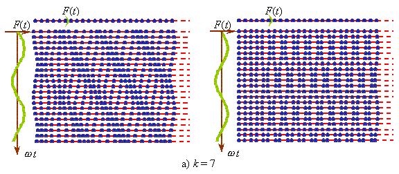
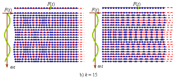
Fig. 4. Diagrams of forced vibrations in a semi-finite homogeneous elastic line in which the external force affects the interior elements of a line. The periodical vibration regime is shown in the left and the aperiodical in the right. The line parameters are m = 0,01 kg; s = 100 N/m; a = 0,01 m; n = 24; F₀ = 0,24 N ;  f = 15 Hz  in the periodical regime; F₀ = 0,06 N ;  f = 31,8 Hz in the critical regime

Going on comparing finite and semi-finite lines, note that at k = 1 , i.e. in case when the force affects the first line element, the solutions (58)- (60) transform into the related solutions of [2] losing the multipliers being specific namely for the given structure of the generalising model, which makes the reverse transition also impossible.

4. The feature of the line heterogeneity at the external force application point

On the considered examples we can run down some common features caused by the external force affecting the line interior elements. In both cases the application point mattered as a heterogeneity on which the vibration pattern transformed. Due to it, in a finite line two sections with different vibration patterns formed. In a semi-finite line there formed a quasi-bounded section with the standing wave, while in an infinite line in [2] there arose two progressive waves propagating in opposite directions, so we may speak about the feature of line heterogeneity at the external force application point.

5. The progressive wave parameters in an infinite elastic line

Studying the features of models for homogeneous elastic lines, we have to note one more peculiarity connected with the parameters of progressive waves propagating along the infinite lumped lines. For these lines the wavelength has quite conventional pattern, because not always it relates to the specific lumped masses. This means, far from always we can select two bodies at a distance of wavelength vibrating in phase. None the less, the body-to-body phase delay equal to 2 indicates also the definite wavelength that fully characterises the line processes.

To determine mathematically, we have to premise that at the distance of a wavelength from a selected element, there exists some fictitious line element vibrating in phase with this selected element of the real line. Noting that, in case of non-damping process, the distance between the elements vibrating in phase does not depend on the amplitude, the wavelength is determined by the expression

On the grounds of (62), the propagation velocity v in the line is determined by the expression

It is typical that in distinction from distributed lines, in the studied models the propagation velocity does not remain constant and depends on the vibration frequency. Therefore, when a complicated-spectral-composition mechanical pulse was fed to the line input, this pulse does not hold its structure when propagating along the line. And only at << 1   the propagation velocity stabilises, coming in the limit to the known value

With it the wavelength will be

which also corresponds to the known value.