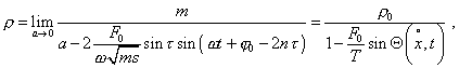
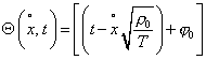
The obtained solution (15) essentially differs from the
known solutions both in amplitude and phase parts. In the amplitude part, instead an
indefinite coefficient A which is known to be the basis of boundary conditions,
the vibration amplitude obtained on the basis of exact analytical solutions is clearly
determined relatively to the frequency  , line density , line density  and line stiffness T. The vibration phase lags from
the external force variation phase by and line stiffness T. The vibration phase lags from
the external force variation phase by  / 2 , which is determined by the complex unity in the right
part of (15). As a result of limit transition the multiplier (2n - 1) in (12) has
transformed into / 2 , which is determined by the complex unity in the right
part of (15). As a result of limit transition the multiplier (2n - 1) in (12) has
transformed into  , and
the trigonometric relationship between , and
the trigonometric relationship between  and and  disappeared; this is non-restorable with the reverse
transition from the distributed line to that lumped. Furthermore, at the limit passing the
parameter is
transformed as disappeared; this is non-restorable with the reverse
transition from the distributed line to that lumped. Furthermore, at the limit passing the
parameter is
transformed as |
Due to this in a distributed line
for the critical ( = 1) and aperiodical ( > 1) vibration regimes the
conditions of their existence will be invalid in the entire range from zero to infinity.
So, should we try making the reverse transition from (15) to (12), using the solutions of
the wave equation to which (15) naturally satisfies, it would fail, the same as we could
not describe the critical and aperiodical vibration regimes. At the same time, to obtain
(15) on the basis of wave equation, we would need to express the initial and boundary
conditions through the parameters of external force and elastic line. However it is known
that we can take as the initial and boundary conditions only numerical values of location
and velocity of the picked out region of an elastic line. Consequently, despite (15)
satisfies the wave equation, we cannot obtain this solution immediately from the equation.
True, in some simple cases one can obtain the solutions for a wave equation having the
right part [16, p. 264- 266], but with the complication of the initial conditions (for
example, in inhomogeneous lines; see, e.g., [17]), or in lines with an elastically fixed
end (see, e.g., [18]) these particular techniques prove to be invalid too. But seeking the
solution by way of limiting process, we will always obtain the exact determined solutions.
On the basis of obtained
solution, determine the regularity of line linear density (t). Note that is strongly real value; it means
that we cannot substitute (12) into (13) immediately. To make a substitution, represent
the external force regularity as |
We see from (19) that, though we
consider in this problem a linear model of an elastic line, (t) has non-sinusoidal, though
periodical pattern. Furthermore, at F0 = T the ruptures form in the
rod, they mean the density discontinuity, and this is unexpected for linear models of such
class of problems that still supposed the absence of any limitations on the affecting
force amplitude or limiting the amplitude by the linearity of rod stiffness T. In
using the approaches based on the determinacy of exact analytical solutions, (19) shows
the upper boundary of allowable load on the line equal to the line stiffness itself. |
 .
.