SELF

30

S.B. Karavashkin and O.N. Karavashkina

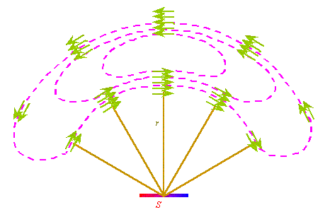
With all accordance of diagrams in Fig. 14 and 15, we have to mark two basic distinctions. First, on the grounds of idea visualised in Fig. 15, we used to conclude that the electric field of transverse wave is closed. In more details, the substantiation is based on the following arguments. "However, how the "momentary photograph" on the whole looks like? It is not difficult to complement it. For it, we have to compare two facts:

1. The field shown in the Figure comes from the transmitter. It had to cover in the void the distance r.

Now the third fundamental fact joins these two. The lines of electric field cannot begin either break somewhere in the void space. We have to complement them so that they become closed curves. We did so in Fig. 16" [13, p. 219].

Fig. 16. Lines of electric field of dipole complemented to the closed field lines [13, p. 220, Fig. 311]

However, as we can see in Fig. 14, there exists no indication to close the electric field on the periphery of dipole radiation. Should such closure took place, then, as it is clearly seen in Fig. 16, together with the transverse component of the field in the region where the field strength vectors turn in the far field, there would be present the longitudinal component. With it, this longitudinal component would not be able to compensate mutually, because, as it is seen in Fig. 16, its appearance is connected with the amplitude fall of transverse field, when the angle of azimuth deviated from the radiation axis of dipole. At the same time, the conventional theory fully denies the longitudinal component in the far field.

Seeking the field closure, we can plot one more dynamic diagram, which would show us the dynamics of variation of the very amplitude of the electric field strength. To plot it, in distinct from Fig. 14, we will not measure the field strength exactly along the radius around the dipole. We will take the transforming grid which we used in the previous item, sequentially put the measuring dipole to all its nodes and measure the field strength in all nodes, keeping the perpendicularity of measuring dipole to the radius-vector from the centre of radiating dipole. With it, for the parameters of half-wave dipole, we will yield the pattern shown in Fig. 17.

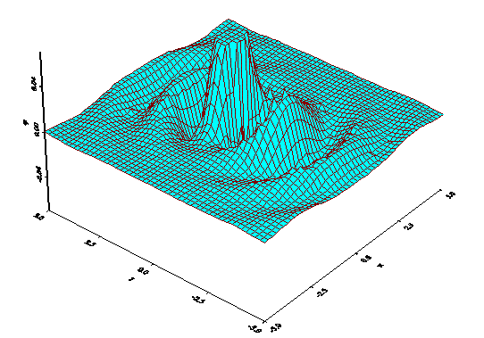
Fig. 17. Dynamic diagram of amplitude of transverse field strength of the half-wave dipole

In this diagram, just as before, the line of dipole charges is parallel to the axis x. The field strength on this axis is fully absent. The maximum of radiation coincides with the normal to the axis of dipole; with it, here we also do not see any features related to the electric field closure. True, we could draw some conventional lines of level, corresponding to the equal values of field strength. Because the diagram is localised around the normal to the dipole axis, these lines of level would be concentric curves, very like those which Pohl presented. But we should not forget, the diagram in Fig. 17 also essentially transforms the pattern of process in the vicinity of dipole, due to specific features of the experimental method described above. The real pattern will have the appearance shown before in Fig. 7, and in this diagram we see no closure of lines of dynamic gradient, though the diagram covers also the far field of dipole radiation.